SCPI and Hardware Instrumentation for Reverse Engineers - Part 1
Introduction
Oscilloscopes, power supplies, and multimeters are all quintessential tools in the hardware hacker's toolbox. While many of us know how to configure these tools manually, I have found that security researchers often overlook the need for remote instrumentation. In this post, we'll outline some basic, practical examples of using SCPI and VISA to instrument the hardware in your lab. In our next post, we'll use these tools in practice to identify SPI signals on a target and extract the contents only using our test equipment.
For this series, I will be using the following equipment:
- MSO 5354 Oscilloscope
- Generic Programmable Power Supply
- FX2LA Based Logic Analyzer
- Saleae Logic Pro 8
Throughout the course of this series, we'll briefly review the protocols that allow us to instrument with our test equipment, provide some basic examples, and finally use them on a practical target. Please note that the commands we are using may differ in your scope, so please be sure to refer to your user manual or programming guide!
SCPI and VISA: A Brief Overview
What is VISA?
VISA is a standard API (Application Programming Interface) for communicating with instruments regardless of the physical interface (e.g., USB, GPIB, RS-232, Ethernet). It provides a unified way to open, configure, and manage communication sessions with instruments. More detailed information about the VISA specification can be found here
VISA is used to open and control connections to our test equipment. For our examples, we will use the PyVisa library to establish communication. With the VISA connection established, we can move on to sending SCPI commands.
Note: VISA functionality is often provided via a third-party library. The PyVisa documentation contains instructions for installing these libraries. However, PyVisa also contains a pure-Python implementation of VISA, which is what we will be using in this post.
What is SCPI?
SCPI is a standardized command set for controlling programmable instruments. This standard is built on top of IEEE 488.2. It defines the syntax and structure of commands sent to instruments and provides a common language for controlling instruments, regardless of the manufacturer.
SCPI commands consist of ASCII characters and contain the following core components.
:- Used to structure the hierarchy of the command?- Indicates that the command is a query, meaning that we expect the instrument to provide a response,- Separates multiple parameters for a given command*- Indicates a “common command” defined by IEEE 488.2
Using these delimiters and components, we can create two different types of commands:
- Set Operations: As the name describes, these are used to set parameters on the target instrument. This includes things like starting captures, configuring channels, and modifying the settings of your instrument
- Query Operations: Query operations are used to request data from your test instrument. Examples of this include querying settings, preparing captured data, and gathering identifying information about your equipment.
The syntax of a query operation is as follows.
:HEADER:SUBHEADER?
For example, to query the current voltage setting on channel 1 of a power supply:
:SOUR:VOLT?
Or to query the vertical scale of an oscilloscope channel:
:CHAN1:SCAL?
The syntax of a set operation can be seen below:
:HEADER:SUBHEADER <value>
For example, to set the voltage output of a power supply to 3.3V:
:SOUR:VOLT 3.3
Or to set the time scale on an oscilloscope to 1 millisecond per division:
:TIM:SCAL 0.001
Note that in the above example a decimal value is provided. Depending on which version of SCPI your test instrument supports you can also provide hexadecimal or binary values with the following prefixes:
- Hex:
#H1D- This will provide
0x1Dto the instrument
- This will provide
- Binary:
#B11011- This will provide
27to the instrument
- This will provide
Some commands require more than one argument; in this case, the arguments are separated by commas as shown in the example below:
:HEADER:SUBHEADER <value1>,<value2>
Short and Long Form Commands
Before we move on, I want to point out that these commands often have abbreviated or "short" forms that require fewer characters. For example, when working with a power supply the command to control power is often documented as:
OUTPut:STATe ON/OFF
In this example OUTPut is the header, STATe is the sub-header and ON/OFF are the available arguments. Often, when looking at SCPI documentation, the lowercase characters in something like OUTPut are optional - meaning that you could send your test equipment:
OUTP:STAT ON
It should also be noted that some commands can be shortened even further - for example output control can also be performed via:
OUTP ON
For more information on command syntax and further examples, check out this Keysight resource, and of course, always check the available documentation for the instrument that you are working with if you run into issues!
How VISA and SCPI Work Together
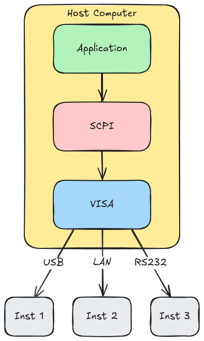
Now that we've talked about VISA and SCPI, let's review how they work together at a high level. SCPI defines the structure of the commands and their syntax, and VISA handles the physical interface through which those commands are sent. The diagram below outlines the relationship between the two:
With our basics and definitions covered, let's review how to set up some of these tools using Python and send some commands to control a power supply!
Setting Up PyVISA
Installation
Depending on your lab environment/requirements there are two ways to utilize PyVisa
pyvisawith backends provided by your instrument manufacturer- Note: See the documentation linked at the beginning of this blog post for specific instructions on building installing specific backends
pyvisa-pywith a generic backend for various instruments.- This is what we'll be using for this post
If you are managing a python project with uv, the dependencies can be installed as shown below:
uv add pyvisa
uv add pyvisa-py
uv add pyserial
uv add psutil
Connecting to an Instrument: VISA Resource Strings
VISA uses resource strings to identify instruments. These strings define how we will be communicating with our test equipment; some examples can be seen in the table below:
| Interface | Resource String Format | Example |
|---|---|---|
| Serial/USB-Serial | ASRL<port>::INSTR |
ASRL/dev/ttyUSB0::INSTR |
| TCP/IP | TCPIP::<ip>::INSTR |
TCPIP::192.168.1.100::INSTR |
| USB TMC | USB::<vid>::<pid>::<serial>::INSTR |
USB::0x1234::0x5678::MY123::INSTR |
| GPIB | GPIB::<address>::INSTR |
GPIB::1::INSTR |
PyVisa gives us the option to connect to a number of different types of resources; these can all be seen in the documentation here.
Basic Connection Example
The following example demonstrates how to use pyvisa to list all available resources:
import pyvisa
# Create resource manager
rm = pyvisa.ResourceManager()
# List available instruments
print(rm.list_resources())
For my hardware setup, I have an oscilloscope connected via Ethernet and a Power Supply that is connected via USB (which presents a serial interface). When I run this, I see the following:
>>> import pyvisa
>>> rm = pyvisa.ResourceManager()
>>> rm.list_resources()
('ASRL/dev/ttyS31::INSTR','ASRL/dev/ttyUSB1::INSTR')
>>>
Note that the Ethernet device did not appear (that's to be expected, don't worry!), but we do see our power supply at /dev/ttyUSB1.
This resource string can be broken down as follows:
- ASRL: Specifies that the resource is an asynchronous serial resource; in this case, the power supply presents a USB to serial device when connected over USB
- Other options include:
TCPIP,PXI, andGPIB, you can see a full list of examples here
- Other options include:
- /dev/ttyUSB1: This contains the path to the instrument that we want to communicate with
- ::INSTR: Specifies that the resource is an instrument. This tells the VISA library that the resource is a device capable of communication using SCPI commands.
Note: The INSTR keyword is required in VISA resource strings to differentiate instruments from other types of resources, such as raw sockets or memory blocks.
Armed with this information, we can attempt to connect to our device and query its identifying information using the built-in query function. This will structure an SCPI query for us and allow us to read the response back from the instrument.
>>> import pyvisa
>>> rm = pyvisa.ResourceManager()
>>> inst = rm.open_resource('ASRL/dev/ttyUSB1::INSTR')
>>> inst.baud_rate = 115200
>>> print(inst.query("*IDN?"))
KIPRIM,DC310S,25012709,FV:V5.2.0
Success! We can now programmatically talk to our power supply. In the next section, we'll cover how to control and configure it using SCPI.
Power Supply Instrumentation
The first SCPI example that we will provide involves power supply instrumentation. This can be useful when running power analysis or fault injection experiments. For our example, our power supply shows up as a USB serial device, so we will connect to it with the following VISA resource string:
res = "ASRL/dev/ttyUSB1::INSTR"
In the next few sections, we'll review what we can do with our power supply via SCPI, but before we do, let's talk about when you might want to instrument your power supply:
- Long Term Testing: If you need to run tests over a long period of time and want to be able to cycle power to your target system automatically
- Physical Proximity: If you're in a lab setting where you aren't directly next to your power supply, you can remotely configure and control your supply using SCPI.
- Automatically Configuring Settings: SCPI allows you to control the current and voltage settings of your power supply. If you're switching targets often and require different voltages, you can use SCPI to program presets and quickly switch between power supply configurations.
- Probing new targets when reverse engineering: One of the first steps of reverse engineering an embedded system involves probing test pads and test points for signals on startup. Manually power-cycling your target can be time-consuming and require a free hand. Automatically cycling power allows you to probe freely with your oscilloscope and continually hunt for interesting signals.
Let's look at some things we can control via SCPI:
Querying Current Settings
We'll start with some commands to read the current settings of our power supply. The commands to query voltage/current and the current output status are:
VOLT?
CURR?
OUTP?
We can issue this in PyVisa using the query function we talked about earlier:
# Query voltage setting
inst.query("VOLT?")
# Query current limit
inst.query("CURR?")
# Query output state
inst.query("OUTP?")
Setting Voltage and Current
Using PyVisa, we can control the settings of our power supply. One of the easiest things to configure is the current voltage and current output settings, as well as the current output state (whether it is on or off ). These commands are shown below:
SOURce:CURRent <unit>
SOURce:VOLTage <unit>
To issue these commands, we can use the write function in PyVisa as shown below:
# Set voltage output to 5V
inst.write("SOUR:VOLT 5")
# Set current limit to 2 A
inst.write("SOUR:CURR 2A")
# Set current limit to .02 A
inst.write("SOUR:CURR .02A")
Enabling/Disabling Output
The OUTP command can be used to turn on or off the power supply's main output.
OUTP:STATE ON
OUTP:STATE OFF
OUTP OFF
OUTP ON
# Enable output
inst.write("OUTP ON")
# Disable output
inst.write("OUTP OFF")
# Query output state
inst.query("OUTP?")
Voltage and Current Limits
We can also set the voltage and current limits on our power supply using SCPI
VOLTage:LIMit VAL
CURRent:LIMit VAL
# Set the voltage limit to 15V
inst.write("VOLT:LIM 15")
# Set the Current limit to 2A
inst.write("CURR:LIM 2")
There are all sorts of things we can control on our power supply. Let's move on to a very simple example that will cycle power to our target while we probe for interesting test points.
Use Case: Automated Power Cycling
This is the simplest example of SCPI. Imagine a scenario where you have an embedded target and are looking for specific signal patterns on startup. You may be looking for an SPI bus that is communicating with a TPM, or you're just hunting for classic UART output. In either scenario, you cycle power every time you want to test a new point on the board, which, after the first fifteen or so tries, can be frustrating!
In this script, we power the target device, wait a few seconds, and then output a chime to let us know we're about to power it down.
Note: Some test equipment will contain SCPI commands to generate chimes, in the past I have used SYST:BEEP:COMP:IMM to play an audible chime when a test is complete. Refer to your instruments' documentation for more information.
for x in range(0,100):
    # Power Target
    inst.write(f'OUTP ON')
    time.sleep(10)
    # Beep to let us know we're about to power down, and we should switch pads
    playsound('beep.mp3')
    # Power off target
    inst.write(f'OUTP OFF')
    time.sleep(5)
Now that we can programmatically cycle power and inform the user of when to switch test points, could we also instrument our oscilloscope to automatically save our captures for later review? Let's talk about oscilloscope instrumentation in the next section.
Oscilloscope Instrumentation
Connection Methods
Much like our power supply, we can also instrument our oscilloscope.
For this example, our oscilloscope is connected to the network and has an IP address of 192.168.1.100
Network/TCP Connection
scope = rm.open_resource("TCPIP::192.168.1.100::INSTR")
Taking Screenshots
Many oscilloscopes allow taking screenshots of the currently captured trace; for this example, we will use the DISP command, as shown in the example below. This example captures the screen state and returns the data in raw binary format as a PNG.
def get_screenshot(inst, filepath):
    """Save oscilloscope display as PNG file"""
    png_data = inst.query_binary_values(':DISP:DATA? PNG', datatype='B', container=bytes)
    with open(filepath, 'wb') as f:
        f.write(png_data)
Notice that for this example, we're using a different function to communicate with our instrument, query_binary_values. This function allows us to make a request to our test equipment and get the resulting data as raw binary. This is useful for screenshots of course, but we can also use it to capture raw trace data! Before we get to that, let's look at how to configure our scope to capture signals via SCPI. In this example, we'll set the vertical scale to 1V and the time scale to 20ms per division.
Channel Configuration Examples
For this post, we'll configure and use channel 1 of the oscilloscope. When working with oscilloscopes, many commands are prefixed with the channel that you want to work with. For example, to test the vertical scale for channel one, we can do the following:
Voltage Scale (Vertical)
# Query current scale
print(inst.query(':CHAN1:SCAL?'))

# Set scale to 1V/div
inst.write(':CHAN1:SCAL 1')
Next, we'll configure the time scale as shown below, check the current timebase, print the response, then set the timebase to 50ms/div.
# Query current timebase
print(inst.query(':TIM:MAIN:SCAL?'))

# Set timebase to 50ms/div
inst.write(':TIM:MAIN:SCAL 0.05')
Finally, with our channel fully configured, we can enable the channel:
# Enable channel 1
inst.write(':CHAN1:DISP ON')
Now that we have our channel enabled, we need to tell the scope how to trigger. What this does is tell our oscilloscope not to begin capturing until we see a specific pattern or the signal crosses a defined voltage threshold. Configuring triggers on an oscilloscope can be confusing at first, but for our example, we'll be using a basic edge trigger. This means that the oscilloscope will not start capturing until it sees the signal cross the edge threshold we configure. In our case, we'll use a falling edge trigger, since the first bit of a standard UART peripheral is the start bit, which is a logical low.
# Set trigger type to edge
inst.write(':TRIG:MODE EDGE')

# Set trigger source to channel 1
inst.write(':TRIG:EDGE:SOUR CHAN1')

# Set trigger level to 1.5V
inst.write(':TRIG:EDGE:LEV 1.5')

# Set trigger edge to falling (for UART start bit)
inst.write(':TRIG:EDGE:SLOP NEG')
Trigger Holdoff
Holdoff prevents re-triggering for a specified time after a trigger event. This can be useful for stabilizing repetitive waveforms, capturing specific frames in serial protocols (SPI, UART), and avoiding triggering on noise/glitches. (The last example is usually what I end up using it for!)
# Set holdoff time
inst.write(':TRIG:HOLD 10E-3')  # 10 milliseconds
With this, we're telling the scope not to trigger again unless it has been at least 10 milliseconds. This will ensure we capture the data on the first trigger.
Capturing Waveform Data
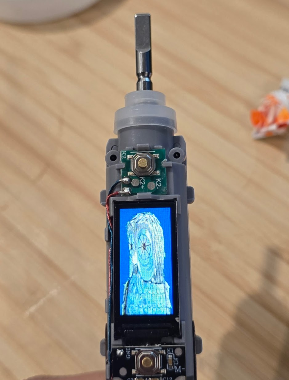
Now that we've configured our trigger and the channel parameters, let's capture a trace and try to save it to our host machine. In this example we are connected to a UART signal on a Smart Thermostat. Given that UART typically idles high (see this post for more information), we will use a falling-edge trigger.
Single Channel Capture
For now, we will set the scope to the single trigger mode, meaning it will trigger once and then stop. This will allow us to capture the data, take a screenshot, and save the signal back to our host machine without worrying about the oscilloscope triggering again.
# Set scope to single trigger mode
inst.write(':SING')

# Wait for the trigger to fire
while inst.query(':TRIG:STAT?').strip() != 'STOP':
    time.sleep(0.5)

# Configure waveform readout
inst.write(':WAV:SOUR CHAN1')
inst.write(':WAV:MODE RAW')
inst.write(':WAV:FORM BYTE')

# Read waveform preamble (contains timing and voltage scale info)
preamble = inst.query(':WAV:PRE?')
print(f"Preamble: {preamble}")

# Read waveform data
raw_data = inst.query_binary_values(':WAV:DATA?', datatype='B', container=bytes)
print(f"Captured {len(raw_data)} data points")

# Save raw data to file
with open('capture.bin', 'wb') as f:
    f.write(raw_data)
Tying It All Together
import pyvisa
import time

rm = pyvisa.ResourceManager()

# Connect to power supply
psu = rm.open_resource('ASRL/dev/ttyUSB1::INSTR')
psu.baud_rate = 115200

# Connect to oscilloscope
scope = rm.open_resource('TCPIP::192.168.1.105::INSTR')

# Verify connections
print(f"PSU: {psu.query('*IDN?').strip()}")
print(f"Scope: {scope.query('*IDN?').strip()}")

# Configure power supply: 3.3V, 500mA limit
psu.write('SOUR:VOLT 3.3')
psu.write('SOUR:CURR 0.5')

# Configure oscilloscope channel 1
scope.write(':CHAN1:DISP ON')
scope.write(':CHAN1:SCAL 0.5')       # 500mV/div
scope.write(':TIM:MAIN:SCAL 0.05')  # 50ms/div

# Configure falling edge trigger for UART start bit
scope.write(':TRIG:MODE EDGE')
scope.write(':TRIG:EDGE:SOUR CHAN1')
scope.write(':TRIG:EDGE:LEV 1.5')
scope.write(':TRIG:EDGE:SLOP NEG')
scope.write(':TRIG:HOLD 10E-3')

# Arm the scope in single trigger mode
scope.write(':SING')

# Power on the target
psu.write('OUTP ON')
print("Target powered on, waiting for trigger...")

# Wait for the scope to trigger
while scope.query(':TRIG:STAT?').strip() != 'STOP':
    time.sleep(0.5)
print("Triggered! Reading data...")

# Take a screenshot
png_data = scope.query_binary_values(':DISP:DATA? PNG', datatype='B', container=bytes)
with open('capture_screenshot.png', 'wb') as f:
    f.write(png_data)
print(f"Screenshot saved ({len(png_data)} bytes)")

# Read waveform data
scope.write(':WAV:SOUR CHAN1')
scope.write(':WAV:MODE RAW')
scope.write(':WAV:FORM BYTE')
preamble = scope.query(':WAV:PRE?')
raw_data = scope.query_binary_values(':WAV:DATA?', datatype='B', container=bytes)
print(f"Captured {len(raw_data)} data points")

# Save waveform data
with open('capture.bin', 'wb') as f:
    f.write(raw_data)

# Save preamble for later analysis
with open('capture_preamble.txt', 'w') as f:
    f.write(preamble)

# Power off the target
psu.write('OUTP OFF')
print("Target powered off. Capture complete!")

# Clean up
psu.close()
scope.close()
rm.close()
If we run this script, we see the following output:
[wrongbaud@mechanicus conduit]$ uv run blog-example.py
PSU: KIPRIM,DC310S,25012709,FV:V5.2.0
Scope: RIGOL TECHNOLOGIES,MSO5354,MS5A250300248,00.01.03.03.00
Target powered on, waiting for trigger...
Triggered! Reading data...
Screenshot saved (1843254 bytes)
Captured 25000000 data points
Target powered off. Capture complete!
[wrongbaud@mechanicus conduit]$
Success, we have data! Including a nice screenshot of our digital signal:
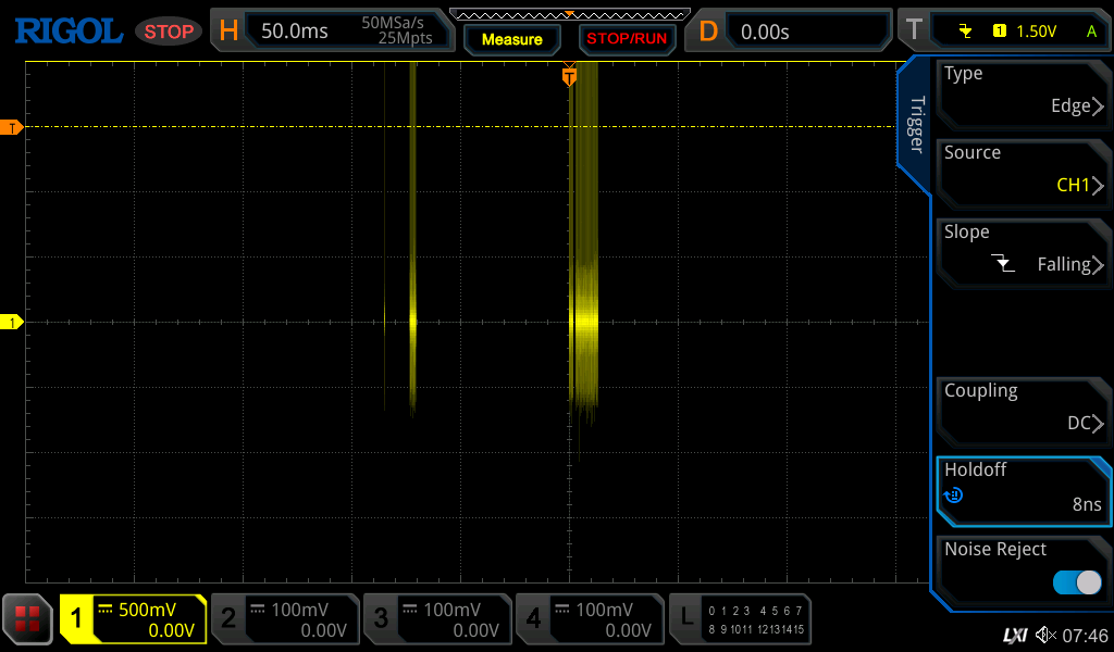
But now that we have this data, how do we import it into other tools for further analysis? While the screenshot is helpful, even to the trained eye, we can tell it is UART, but it doesn't give us much for low-level analysis. In the final section of this post, we'll review how to import this data into pulseview.
Loading Captures into PulseView
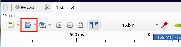
Now that we have captured what we think is a UART signal, let's load it into PulseView to get a closer look. Remember that we have a raw binary capture; it hasn't been formatted for a logic analyzer to understand. Luckily for us, PulseView can import raw analog captures. To do this, first select the Open Icon:
Next, select Import Raw Analog Data Without Header, which will open a file browser. For this example, we'll select the trace we just captured. Once a trace is selected, the following prompt will appear.
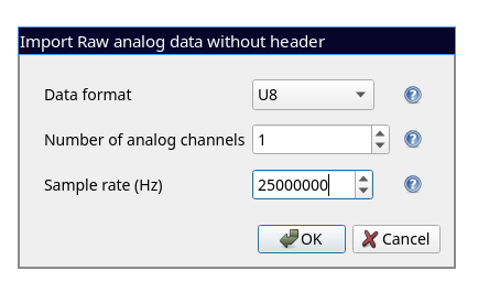 For this example, we will specify the data format to be
 U8 and for the sample rate, we can either look at the current scope settings or we can use the preamble text that we extracted from the device:
0,2,25000000,1,2.000000E-8,-2.500000E-1,0.000000,2.0587E-02,0,128
The third field is our sample rate: 250000000, which is 25 Mpt/s. When we use these settings, we see the following:
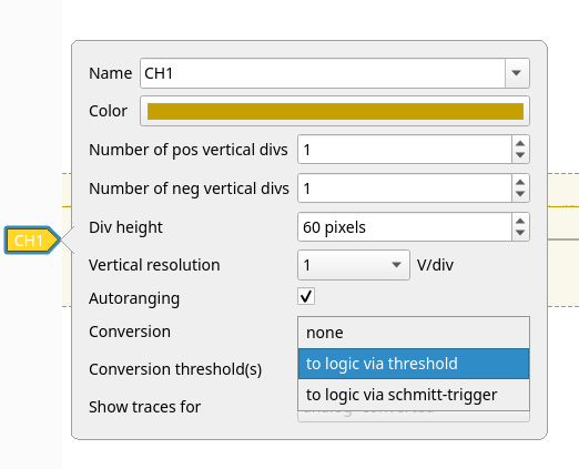
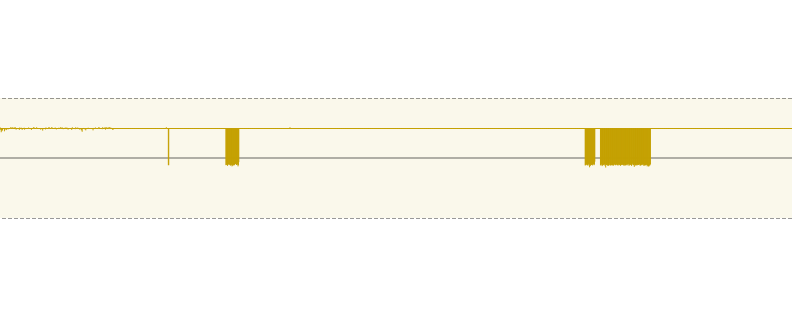 Here is our analog signal in Pulseview! But we need to configure pulseview to convert these analog pulses into digital values. In PulseView, there are several ways to convert your analog capture into digital pulses. For this example, we will select our channel
 CH1 and use the Logic via Threshold setting as shown in the image below:
 Now, when we look at our signal, it has been properly converted:
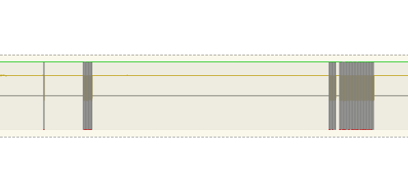
Now we can leverage all of pulseview's decoders and analysis capabilities to examine the digital signal we captured with the oscilloscope. Given that we think this is a UART we can measure the first low pulse that we see and calculate the frequency:
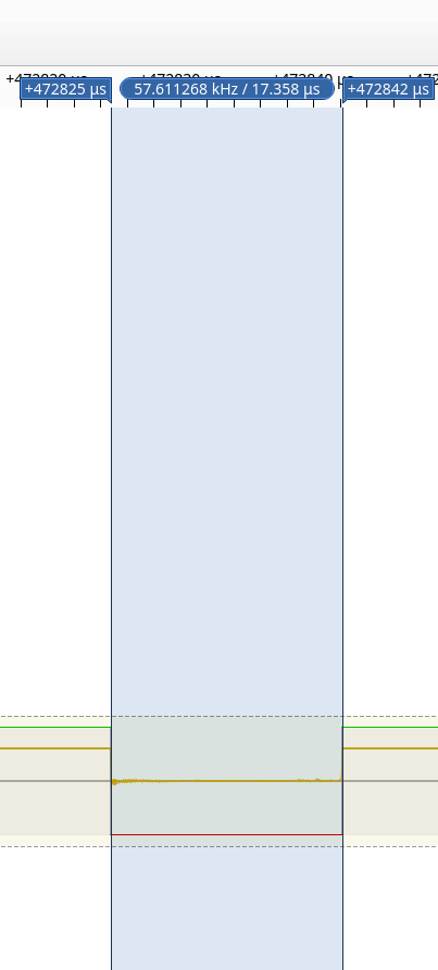 This shows that we have a frequency of 57.611268 kHz, or approximately 57,600 bits per second!
Note: If you want a deep dive on calculating baud rates on an unknown UART, check out our blog posts here and here
After setting up the decoder, we see the following data:
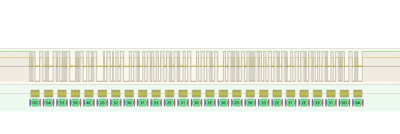
And if we zoom out on this we have:
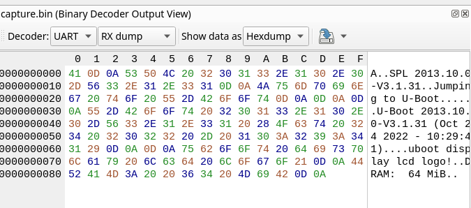
And with that - we've found a UART! We successfully instrumented both the power supply and the oscilloscope to extract UART data from this target. In the next post, we'll do a proper hardware teardown and take a look at some more complex signals!
Conclusion
In this post, we've talked about the basics of SCPI and visas, and how you can use them to aid reverse engineering. Not only does having an understanding of SCPI and VISA help when you're physically far away from your test equipment, but it also helps you document your findings by capturing traces and saving screenshots of interesting signals!
If you want to learn more about SCPI/VISA check out our repository with some basic examples that utilize the PyVisa library here We've put together a wrapper for basic oscilloscope control and power supply control, see the repository for more details!
In part two of this post, we'll look at more complex, multi-channel examples and discuss how to load multiple captures into pulseview for signal analysis.
Lastly, if you're looking to learn more about hardware reverse engineering, check out our roadmap of free resources here. If you're interested in structured training for your team, check out our hardware hacking bootcamp. If you're looking for an in-depth dive into how hardware-level debuggers work and how to reverse engineer them, check out our self-paced course here.
If you want to stay informed about official releases, new courses, and blog posts, sign up for our mailing list here.
Thanks for reading - and happy hacking!
Matt